Contribution function and formation height of 854.2

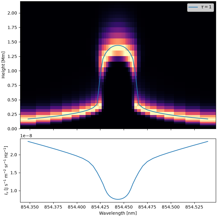
After converging a simulation, the depth-dependent opacity and emissivity can be stored during a formal solution, and used to compute optical depths and contribution functions. Here we look at where the Ca II 854.2 nm line forms in the FAL C atmosphere.

import matplotlib.pyplot as plt
import numpy as np

import lightweaver as lw
from lightweaver.fal import Falc82
from lightweaver.rh_atoms import CaII_atom, H_6_atom
from lightweaver.utils import compute_contribution_fn, compute_tau, tau_isosurface

Converge the NLTE problem with H and Ca II active.

atmos = Falc82()
atmos.quadrature(5)
rad_set = lw.RadiativeSet([H_6_atom(), CaII_atom()])
rad_set.set_active('H', 'Ca')
spect = rad_set.compute_wavelength_grid()
eq_pops = rad_set.compute_eq_pops(atmos)
ctx = lw.Context(atmos, spect, eq_pops, Nthreads=2)
lw.iterate_ctx_se(ctx, quiet=True)

240

Ask the formal solver to store the full depth-dependent opacity and emissivity (ctx.depth_data), then perform one more formal solution.

ctx.depth_data.fill = True
ctx.formal_sol_gamma_matrices()

IterationUpdate(ctx=<lightweaver.Context object at 0x558d19ff3f30>, crsw=1.0, updated_J=True, dJ_max=0.004928092666125372, dJ_max_idx=308, updated_pops=False, dpops=[], dpops_max_idx=[], ng_accelerated=False, updated_ne=False, dne_max=0.0, dne_max_idx=0, updated_rho=False, Nprd_sub_iter=0, drho=[], drho_max_idx=[], updated_J_prd=False, dJ_prd_max=[], dJ_prd_max_idx=[])

Compute the contribution function and optical depth for the outgoing ray with the largest mu (the last ray of the quadrature), and the height at which tau = 1 along this ray. These are computed for every wavelength of the simulation’s grid, so we select the points around 854.2.

mu = -1
cfn = compute_contribution_fn(ctx, mu=mu)
tau = compute_tau(ctx, mu=mu)
z = np.asarray(atmos.height)
tau1 = tau_isosurface(tau, z)

wavelength = np.asarray(ctx.spect.wavelength)
ca_8542 = 854.444
mask = np.abs(wavelength - ca_8542) < 0.1
wave = wavelength[mask]
I = np.asarray(ctx.spect.I)[mask, mu]

Integrating the contribution function over height gives the emergent intensity (up to the accuracy of this simple quadrature).

integrated = -np.trapezoid(cfn[mask], z, axis=1)
print(
    f'Max relative difference between integrated cfn and I: '
    f'{np.max(np.abs(integrated - I) / I):.2e}'
)

Max relative difference between integrated cfn and I: 5.48e-02

Plot the contribution function (normalised at each wavelength) with the tau = 1 height overlaid, and the emergent profile below. The line core forms in the chromosphere, around 1.2 Mm higher than the wings.

z_mm = z / 1e6
fig, ax = plt.subplots(
    2, 1, figsize=(7, 7), sharex=True, height_ratios=[2, 1], constrained_layout=True
)
cfn_norm = cfn[mask] / cfn[mask].max(axis=1, keepdims=True)
ax[0].pcolormesh(wave, z_mm, cfn_norm.T, shading='auto', cmap='magma')
ax[0].plot(wave, tau1[mask] / 1e6, c='C0', label=r'$\tau = 1$')
ax[0].set_ylim(0, 2.2)
ax[0].set_ylabel('Height [Mm]')
ax[0].legend()
ax[1].plot(wave, I)
ax[1].set_xlabel('Wavelength [nm]')
ax[1].set_ylabel(r'$I_\nu$ [J s$^{-1}$ m$^{-2}$ sr$^{-1}$ Hz$^{-1}$]')
plt.show()