Time-dependent Example

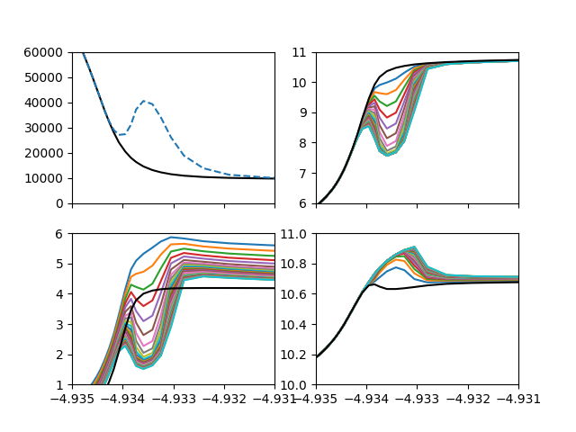
Simple illustrative example of time-dependent method. Herein we reproduce the time-dependent population figure present in Judge 2017. Here the complete Rybicki-Hummer MALI method is used. Herein we also conserve charge.

Judge (2017): ApJ 851, 5

from lightweaver.fal import Falc82
from lightweaver.rh_atoms import  H_4_atom, C_atom, O_atom, Si_atom, Al_atom, CaII_atom, Fe_atom, He_atom, MgII_atom, N_atom, Na_atom, S_atom
import matplotlib.pyplot as plt
import time
import numpy as np
import lightweaver as lw

/home/runner/work/Lightweaver/Lightweaver/lightweaver/config.py:75: UserWarning: No config file found, using defaults. For optimised vectorised code, please run `lightweaver.benchmark()`, otherwise the most advanced instruction set supported by your machine will be picked, which may not be the fastest (due to e.g. aggressive AVX offsets).
  warnings.warn('No config file found, using defaults. For optimised vectorised code,'

Set up the standard FAL C 82 point initial atmosphere.

atmos = Falc82()
atmos.quadrature(5)
aSet = lw.RadiativeSet([H_4_atom(), C_atom(), O_atom(), Si_atom(), Al_atom(), CaII_atom(),\
                        Fe_atom(), He_atom(), MgII_atom(), N_atom(), Na_atom(), S_atom()])
aSet.set_active('H')
spect = aSet.compute_wavelength_grid()

eqPops = aSet.iterate_lte_ne_eq_pops(atmos)
ctx = lw.Context(atmos, spect, eqPops, conserveCharge=True, Nthreads=1)

Find the initial statistical equilibrium solution,

lw.iterate_ctx_se(ctx)

print('Achieved initial Stat Eq\n\n')

-- Iteration 0:
dJ = 1.00e+00
    (Lambda iterating background)
-- Iteration 4:
dJ = 9.64e+00
    H delta = 1.0905e+00
    ne delta = 1.6015e-01
-- Iteration 29:
dJ = 8.46e-02
    H delta = 5.1054e-02
    ne delta = 7.0413e-16
-- Iteration 54:
dJ = 5.37e-02
    H delta = 3.2221e-02
    ne delta = 2.7092e-16
-- Iteration 79:
dJ = 1.85e-02
    H delta = 1.2072e-02
    ne delta = 1.7016e-16
-- Iteration 103:
dJ = 3.29e-03
    H delta = 2.1979e-03
    ne delta = 6.8064e-16
--------------------------------------------------------------------------------
Final Iteration: 113
--------------------------------------------------------------------------------
dJ = 1.45e-03
    H delta = 9.6901e-04
    ne delta = 7.0413e-16
--------------------------------------------------------------------------------
Context converged to statistical equilibrium in 113 iterations after 2.51 s.
--------------------------------------------------------------------------------
Achieved initial Stat Eq

Simulation parameters, timestep, number of steps to run for, and how many times to attempt to solve the equations for convergence per step.

start = time.time()
dt = 0.1
NtStep = 30
NsubStep = 100

Perturb the atmospheric temperature structure like in the paper.

prevT = np.copy(atmos.temperature)
for i in range(11, 31):
    di = (i - 20.0) / 3.0
    atmos.temperature[i] *= 1.0 + 2.0 * np.exp(-di**2)

Solve the problem

hPops = [np.copy(eqPops['H'])]
subIters = []
for it in range(NtStep):
    # Recompute line profiles etc to account for changing electron density and temperature.
    ctx.update_deps()

    prevState = None
    for sub in range(NsubStep):
        JUpdate = ctx.formal_sol_gamma_matrices()
        # If prevState is None, then the function assumes that this is the
        # subiteration for this step and constructs and returns prevState
        popsUpdate, prevState = ctx.time_dep_update(dt, prevState)
        # Update electron density.
        # If conserveCharge is set to True when the context is constructed, then
        # the effects of `time_dep_update` are included in the IterationUpdate
        # returned from `nr_post_update`, as the Context is expecting this to be
        # called immediately after `time_dep_update`.
        nrUpdate = ctx.nr_post_update(timeDependentData={'dt': dt, 'nPrev': prevState})

        # Check subiteration convergence
        if nrUpdate.dPopsMax < 1e-3 and JUpdate.dJMax < 3e-3:
            subIters.append(sub)
            break
    else:
        raise ValueError('No convergence within required Nsubstep')

    hPops.append(np.copy(eqPops['H']))
    print('Iteration %d (%f s) done after %d sub iterations' % (it, (it+1)*dt, sub))

    # input()
end = time.time()

Iteration 0 (0.100000 s) done after 51 sub iterations
Iteration 1 (0.200000 s) done after 48 sub iterations
Iteration 2 (0.300000 s) done after 46 sub iterations
Iteration 3 (0.400000 s) done after 41 sub iterations
Iteration 4 (0.500000 s) done after 36 sub iterations
Iteration 5 (0.600000 s) done after 30 sub iterations
Iteration 6 (0.700000 s) done after 30 sub iterations
Iteration 7 (0.800000 s) done after 24 sub iterations
Iteration 8 (0.900000 s) done after 22 sub iterations
Iteration 9 (1.000000 s) done after 21 sub iterations
Iteration 10 (1.100000 s) done after 19 sub iterations
Iteration 11 (1.200000 s) done after 18 sub iterations
Iteration 12 (1.300000 s) done after 17 sub iterations
Iteration 13 (1.400000 s) done after 17 sub iterations
Iteration 14 (1.500000 s) done after 16 sub iterations
Iteration 15 (1.600000 s) done after 16 sub iterations
Iteration 16 (1.700000 s) done after 20 sub iterations
Iteration 17 (1.800000 s) done after 21 sub iterations
Iteration 18 (1.900000 s) done after 14 sub iterations
Iteration 19 (2.000000 s) done after 13 sub iterations
Iteration 20 (2.100000 s) done after 13 sub iterations
Iteration 21 (2.200000 s) done after 12 sub iterations
Iteration 22 (2.300000 s) done after 11 sub iterations
Iteration 23 (2.400000 s) done after 11 sub iterations
Iteration 24 (2.500000 s) done after 10 sub iterations
Iteration 25 (2.600000 s) done after 9 sub iterations
Iteration 26 (2.700000 s) done after 9 sub iterations
Iteration 27 (2.800000 s) done after 8 sub iterations
Iteration 28 (2.900000 s) done after 7 sub iterations
Iteration 29 (3.000000 s) done after 7 sub iterations

Reproduce Judge plot.

initialAtmos = Falc82()

plt.ion()
fig, ax = plt.subplots(2,2, sharex=True)
ax = ax.flatten()
cmass = np.log10(atmos.cmass/1e1)

ax[0].plot(cmass, initialAtmos.temperature, 'k')
ax[0].plot(cmass, atmos.temperature, '--')

for p in hPops[1:]:
    ax[1].plot(cmass, np.log10(p[0,:]/1e6))
    ax[2].plot(cmass, np.log10(p[1,:]/1e6))
    ax[3].plot(cmass, np.log10(p[-1,:]/1e6))

p = hPops[0]
ax[1].plot(cmass, np.log10(p[0,:]/1e6), 'k')
ax[2].plot(cmass, np.log10(p[1,:]/1e6), 'k')
ax[3].plot(cmass, np.log10(p[-1,:]/1e6), 'k')

ax[0].set_xlim(-4.935, -4.931)
ax[0].set_ylim(0, 6e4)
ax[1].set_ylim(6, 11)
ax[2].set_ylim(1, 6)
ax[3].set_ylim(10, 11)

print('Time taken: %.2f s' % (end-start))

Time taken: 6.14 s