Thyr
Simulating Microwave Emission from Solar Flares
Chris Osborne (2087801)
Project Aims
Increased resolution simulation of microwave (MW) emission from flares, in particular the foot regions.
- Not resolvable by modern radio astronomy equipment.
- Produce an initial idea of what we may see.
Focus on gyrosynchrotron (GS) emission.
- First analytically described by Ramaty in 1969.
- Mildly relativistic electrons (\(\gamma \sim 5\)) spiralling through a magenetic field.
GS Simulation
- Computer simulation of GS Emission is not a new idea.
- First program produced by Ramaty in an early FORTRAN.
- We can directly trace our lineage back to that program.
Computer Simulation
- Why now?
- Solve numerically not analytically
- Modern computers are many orders of magnitude more powerful than when Ramaty wrote his original simulation.
- Can afford to be "profligate" with computational resources (within reason)
- The simulation of \(j\) and \(k\) is typically less than 50ms per frequency - on this laptop!
Design: Start with Previous Developments...
Output from PJAS' gyro3d (IDL)
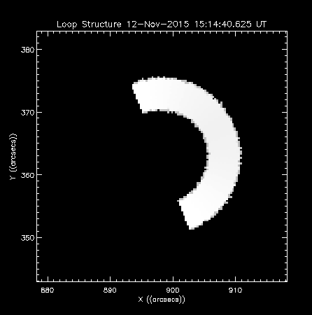
Design: ...And the Desired Output
An emission map plotted in MATLAB.
Main Methods
GS Simulation as per PJAS' modified version of Ramaty's code, given a quick optimisation pass
Volumetric Raytracing
Original aim was to provide arbitrary flare geometry
- This proved harder than expected, provided highly adjustable loop instead.
- How adjustable?
Our Loop Model
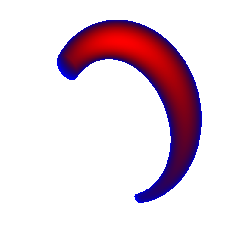
Our modified torus presenting a flare shape with −20\(^{\circ}\) lean, at latitude 30\(^{\circ}\) and longitude 70\(^{\circ}\). The shape also presents a 30\(^{\circ}\) back angle and 40\(^{\circ}\) asymmetry or inclination.
Programming Model
Extensible modular modern C++ core
Interpreted full featured Lua scripting front-end.
- Acceptable speed - within factor of 5 of C for double precision maths.
Unless modifying the software beyond its design role, most users should never have need to touch the C++.
Extensive documentation and examples for the front-end (See users manual). API reference provided for the core.
MATLAB script (available in the user's manual),
but these are also easily creatable with free software such as gnuplot, using the following
script:
set terminal pdf color
set datafile separator ","
set output "Colormap.pdf"
set key off
set xrange [0:800]
set yrange [0:800]
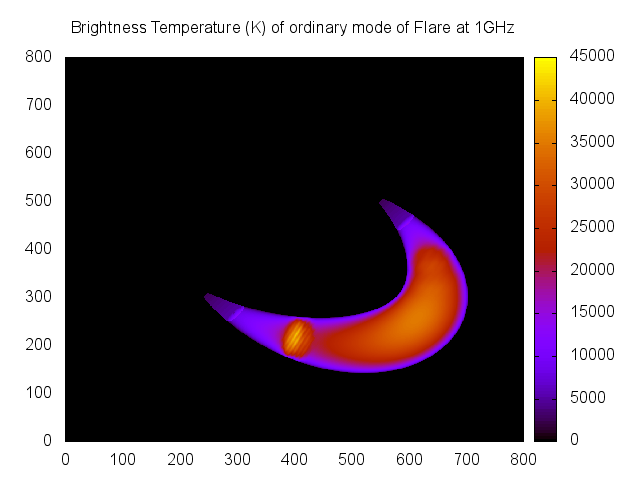
set title "Brightness Temperature (K) of ordinary mode of Flare at 1GHz"
plot "th.1.000000GHz.O.csv" matrix with image
This can easily be meta-programmed using bash, python, perl etc. to automatically fill in the
graph titles from the filenames, much as the MATLAB script does.
IDL also works well for this task, as does R for more in-depth statistical processing.
Sample Gnuplot output
Example
function ArcToCMSun(h)
   -- DegToRad / "perDeg * AstroUnit
   return math.pi / 180.0 / 3600.0 * 1.49597870e13 * h
end

function CMSunToArc(h)
   return h / (math.pi / 180.0 / 3600.0 * 1.49597870e13)
end

densityScaleHeight = CMSunToArc(130e5);
kappa = 10
loopDensity = 10e9
photDensity = 1.16e17

function BMagnitude(s)
   if (math.abs(s) > highResRadialPos) then
      return 600 + ((20 * math.abs(s) - highResRadialPos)
            / (1- highResRadialPos))^2
   else
      return 200 + ((20 * math.abs(s))
            / highResRadialPos)^2
   end
end

function PlasmaDensity(h)
   if (h < highResHeight) then -- roughly based on Battaglia et al. ApJ 752
      local nExp = loopDensity + photDensity * math.exp(-h / densityScaleHeight)
      local nk = photDensity * (1 + h / (kappa * densityScaleHeight))^(-kappa + 1)
      return nExp + nk
   else
      return 1.0e9
   end
end

function Temperature(h)
   if (h < highResHeight) then
      return 5000 + 5000 * (h / highResHeight)
   else
      return 2.0e7
   end
end

function NonThermalDensity(s)
   return 1.0e6
end

function Delta(s)
   return 4.0
end

function EnergyMinMax(s)
   return 10, 5000
end

RT.SetViewportSize(25,25)
RT.AddLoop('l1')
l1.SetSolarSize(8, 2, 0.2)
l1.SetSolarLoc(0, 60, 40, 70)
l1.SetHighRes(2, 2)
l1.SetDomains(20)
RT.CullDomains()
RT.LoadFreqList('logFreqs.csv')
RT.GUpdate()
RT.SaveAllCSVs('flare1')
Interface
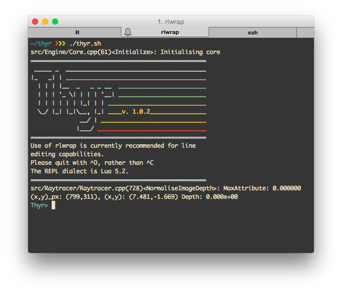
Interface
- Previous slide showed interactive interface.
- Can also be run with pre-written scripts.
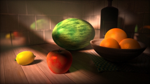
Demonstration
Current Compromises
Raycasting against large number of domains
- Currently \(O(N^3)\), could be \(O(N\log(N))\) using octree sorting.
- Time to implement: < 7 days.
- Look at Ogre3D/Urho3D/my Lethani for source inspiration.
Alternative: Replace current domain system with something like BSP
- Time to implement $\sim$1 month. See Quake/Unreal Engine source.
Current Compromises
- Only single power law electron distribution available in Lua.
- The back-end is already in place for multi-power law, we just need a way to link the two.
- Time to implement: < 3 days.
Current Compromises - A comment
The most time-consuming part of the GS simulation is the Bessel function calculations. These are responsible for peaks in the emission spectrum, however it may be a good idea to use an interpolation scheme depending on the precision that is actually required.
Investigation required.
Further Possibilities
Other geometry types
- The algorithms used are applicable to any shape - if it can't be parametrised directly, then we can use polygons.
- Time to implement: $\sim$2 weeks. See raytracers (e.g. POVRay).
Other frequency ranges
- If \(j\) and \(k\) can be calculated for the cloud/plasma, we can use it.
- Should be a fairly minor modification < 10 days to add a second frequency range (e.g. EUV), faster from there.
The above would require slight modifications of currently hard-coded constants if non-solar bodies were to be analysed.
Further Possibilities
- Allowing the user to define different functions per flare in the multi-loop case.
- Time to implement: < 4 days
Further Possibilities
- Modern raytracing techniques (raymarching)
- These techniques could massively increase the resolution and complexity of shapes while improving speed and decreasing memory usage (GPGPU).
- Time to implement: Probably at least 2 months.
Raymarching
Made by Íñgo Quílez, using a 4KB binary, no external files, renders on a 4 year old GPU in near real time.
Interesting developments
- A more in-depth survey of the possible variations of parameters that could lead to heavy GS emission from the flare foot points (and estimating its magnitude)
- Presumably a combination of high density with increased temperature relative to the chromosphere.
Interesting developments
- Reanalysing the situation set up in (Simões & Costa 2006) using a multi-loop model with more accurate chromospheric and coronal temperature and density models. Hopefully allowing a direct comparision to NoRH and RHESSI data, thus confirming the validity of the models.
Acknowledgements
I would like to thank Dr. Simões (my advisor), and the University of Glasgow Astronomy department for supporting me and funding this project. I also wish to thank all the coders whose previous work has been invaluable.
Please also see the user's manual and my summer report.
Questions?